Binary Classifier
This post will explain how binary classifiers were used to classify excerpts from news articles about shooting events. The classes for classification were:
- Class 1 Accountability: if the excerpt is talking about accountability related to the shooting, i.e. who or what was responsible
- Class 0 Not accountability: if the excerpt is not talking about accountability.
The three shooting events described in the news articles were Isla Vista, Marysville and Newtown. This post will explain the experiment and the results of some simple baseline classifiers to identify these classes.
Text representation
The first step in a natural language processing (NLP) classification task, is to transform the text into a numerical vector representation. There are many ways to do this, but for this experiment two basic text representations are used: the count vector and the Term-Frequency Inverse Document frequency (tfidf) vector. These vectors will both use the “bag of words” representation, where each document is “tokenized” into a list of the individual words it contains, and the counts of these tokens are used to determine the vector for each document. The tokens from the full dataset is used to build the vocabulary.
Tokenization
In order to transform the document into a vectorized representation, first it must be divided into the units called tokens. For example, if the sentence is “The dog chases the ball.”, the tokens would be: The, dog, chases, the, ball. Next, each token is stemmed, and converted to lower case, to result in: the, dog, chase, the, ball.
Count Vector
The count vector approach represents each document by the count of each word (token) it contains. Each document can be represented by a vector of the length of the full vocabulary of all the documents, and each word will be represented by the count of the number of times that word occurs in the document. As a result, most of the vectors for each document will be 0s, since the total vocabulary across all documents will be much greater than the number of words contained in one individual document.
Tfidf vector
An alternative vector commonly used to represent documents is called the “Term- frequency Inverse-Document-frequency” (tfidf) vector. The first step for this, is once again tokenization, but the document vectors are not represented directly by the count of each word. This vector weights each word based on its frequency in the document, and inversely proportional to its frequency across all documents. This will result in providing a lower weight to words that are very common across all documents, for example “the”. The word “the” probably does not carry a lot of document specific meaning even if it has a high count within the document. Representing a document by the tfidf vector will give a higher weight to the words that have a high count in that document relative to the rest of the documents.
Baseline Classifiers
It is important to establish baselines with simple models, since there is often a trade-off between model interpretability and accuracy. Jumping right to a more complex model can result in slow run time to train the models that may be unnecessary. Also, it will be harder to determine and explain where the model is going wrong, and what could be done to improve the performance in more complex models. It is important to know what levels of accuracy can be achieved with the simple, fast and interpretable models. This can be used to establish performance baselines, and in the future any added complexity in either the text representation or the classification method should be justified by an increase in performance over these baselines.
Linear Classifiers
Two common linear classifiers were used: support vector machines and logistic regression. Both of these separate the documents, which are represented by high dimensional vectors, by a hyperplane. The coefficients of the hyper-plane can indicate which features are most important in making the decision about which class a document belongs to
Ensemble Classifiers
An ensemble method was also tested, called random forest, which is a an ensemble of decision trees. This model creates a more complicated boundary separation, but the sklearn implementation can still track the importance of each feature (token) in making the decision about which class a document belongs to.
Experiment
The documents were first processed by tokenization, stemming, converting all words to lower case, and removing standard “stop words” (stop words are words that are very common and prevalent across all english documents, e.g. “the”, “and”, etc.). Next, the documents were vectorized using the the count vectorizer and the tfidf vectorizer. Each of these representations was tested with each of the three mentioned classifiers, to result in a total of six models being fit and tested. The best vector type for each classifier was saved, and the best results were also saved.
Results
Full Data
The results on all three shooting datasets from all six models were very similar, but the results from support vector machine (svm) using the count vectors was the best. The results were:
Confusion matrix:
[[3627  143]
 [ 215  390]]

 Classification Report:
              precision    recall  f1-score   support

           0       0.94      0.96      0.95      3770
           1       0.73      0.64      0.69       605

    accuracy                           0.92      4375
   macro avg       0.84      0.80      0.82      4375
weighted avg       0.91      0.92      0.92      4375
Isla Vista
The same procedure was repeated on Isla Vista data alone. The results were better than the full dataset, and the best model was random forest with the tfidf vectors.
Confusion matrix:
[[1224   22]
 [  87  293]]

 Classification Report:
              precision    recall  f1-score   support

           0       0.93      0.98      0.96      1246
           1       0.93      0.77      0.84       380

    accuracy                           0.93      1626
   macro avg       0.93      0.88      0.90      1626
weighted avg       0.93      0.93      0.93      1626
The main thing to note in these results is the imbalance in the confusion matrix between the false positive and the false negatives. The false positives for accountability (22) were much lower than the false negatives (87). This could be due to the fact that overall there are much fewer documents that were labelled as accountability than documents that were not labelled. The number 1224 corresponds to the number of non-accountability excerpts that were labelled as non-accountability (true negative), and the 293 is the number of accountability documents labelled as accountability (true positive).
Most Important Features
The most important features for the svm on the full data set is shown in the figure below. The positive blue bars show which words are most influential to result in a classifying an excerpt as accountability, and the negative red bars most influential to classify as non accountability.
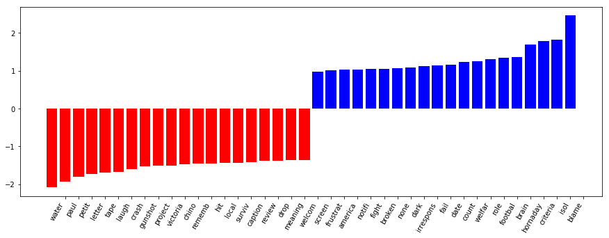
It is nice to observe that the word “blame” is the highest word contributing to classification as accountability.
Error Analysis
We can inspect some examples of where the classifier is going wrong, by looking at some examples of where it guesses the document was about accountability when actually it was not (false positive), and also where the model predicted a document to not be accountability when actually it was (false negative).
False Positive examples
The following are some excerpts that were incorrectly predicted as accountability. The terms that may have mislead the classifier to classify these excerpts as accountability are indicated in blue (corresponding to the feature importance plot).
“Many of the students at UCSB blame the media, insisting the nonstop coverage rewards the murderer in death with the attention and “fame” he sought in life.”
This example contains the word “blame” which is a strong indicator of the accountability label. Reading this excerpt, it does seem like it could be related to accountability. This example shows that this is a complex task, even to human judgement.
“The Washington Post offered an excellent example of this over the weekend, when Ann Hornaday argued that the real culprit for Eliot Rodger’s murder spree was … Judd Apatow, James Bond and a bad Robert Downey flick that probably only Hornaday remembers.”
This example is a bit less clear than the previous, and the word that probably lead to mis-classification as accountability was “Hornaday”. This example does seems somewhat related to accountability as well, mentioning that the real culprit for the crime is movies that portray guns in positive way.
“I spent a lot of last weekend fighting tears as I contemplated this most profound of questions.”
This example was likely mis-classified as due to the presence of the word “fight”. This example seems to be very unrelated to accountability, and this demonstrates the limitations of the bag of words representation. It is likely that this phrase could not be classified well with any complex classifier with more complex decision boundaries, without first improving the input representation of the text to capture more meaning than is preserved with the simple bag of words method.
False Negative examples
The following are some excerpts that were incorrectly not predicted as accountability. The words with a strong weight towards non-accountability are indicated in red.
“His mother knew he was a danger to himself and others and asked the local cops to pay him a visit. The police did go to the kids apartment, but saw no reason to lock him up.”
This example seems a bit questionable how it relates to accountability, and so this is another example of where a non-expert may have just as much trouble identifying accountability as this classifier does. It seems it does relate somewhat to blaming the police, though once again this will be tricky to capture this only based on the words present in the bag of words representation.
“The ban, which expired in 2004, would certainly have made a difference in the number of children who survived the Newtown shooting. The shooter could not have shot as many, as quickly, as he did.”
This excerpt seems to more clearly related to accountability, and was likely missed by the classifier due to the presence of the word “survive”, which is in general a more positive word and likely used less often when talking about accountability for the crime of the shooting.
“The next time you want to call a woman a derogatory term because she doesn’t show any interest in you, take a step back and remember thats the kind of thinking that caused Rodger to go off on his tantrums.”
This example does seem to pretty clearly refer to accountability when it states “the kind of thinking that caused …” and so it seems the algorithm could be improved by paying more attention to the mention of the word caused, and also by capturing more meaning in the structure of the sentence when talking about causality.
Conclusions
The main conclusions from these results so far, is that the choice of classifier seemed to make minor impact on the results, with the f1 scores across all models tested varying by only 0.02 (full results shown in the jupyter notebook on github).
Based on assessment of errors, it seems there is much improvement to be gained by improving the text representation to include features that capture more meaning than can be captured with individual words in the bag of words model.